A Real-Time Ballistics Calculator

This is the story behind KOBE (Kinetic Optimizer for Ballistic Engagements), and how I was able to achieving blazingly fast performance after borrowing some tricks from video game rendering algorithms.

Background

Why?

I attended an Australian Defense Force Hackathon and conference last year, and it was very evident that almost everyone was interested in one thing in particular; Drones. This isn’t without good reason: these devices allow operators to remotely surveil, track, and perform advanced reconnaissance on targets from kilometers away. This is why they are so prevalent in the Russia/Ukraine war where both sides have developed counter-measures and counter-counter-measures for everything from $200 quadcopters to $30 million dollar Reapers.

I wanted to offer a unique advancement to this field and found my calling when I saw that almost every single open source ballistics calculator is painfully slow. So what if we write our own solution in Rust?

This is a story that summarizes decades of ballistics advancements (or at least, whatever was declassified), cool low level tricks, and creating the first ever real-time ballistics calculator that can run four orders of magnitude faster than the current best.

What Makes a Bullet Move

While ideally we would be able to describe everything as *what comes up, must go down*, we start encountering some issues with ‘the thing’ when it’s moving faster than the speed of sound and rotating up to 5,000 rotations per second.

As a brief summary of what to look out for (other than gravity), we have the following ‘gotchas’:

Factor	Description
Drag	Air resists motion, and resistance increases with the square of velocity. This becomes more complicated when the projectile approaches the speed of sound, which we’ll explore in the next section.
Wind	Is actually quite simple and can be accounted for within the drag equations by subtracting wind velocity from the projectile’s velocity to compute relative speed.
Spin Drift	This is dependant on quite a few forces, and depending on who you ask you’ll get a different answer. One common explanation is that the spinning bullet “rolls” off the cushion of air formed beneath it, but it’s also due to gyroscopic forces as the spinning bullet follows a parabolic trajectory due to gravity.
Coriolis Effect	Extremely minor but present. The Earth’s rotation causes slight deflection during flight. Insignificant for most shooting but relevant at extreme ranges.

A Side Quest: Drag Models

If you ask around, you’ll quickly find out that drag is the bane of almost any physicist’s existence. Unlike gravity, air can be compressed and likes to ‘grip’ onto surfaces, causing turbulence and chaotic activity.

This might be somewhat surprising, especially when the drag equation looks deceptively simple:

F_drag = 0.5 * p * v * v * Cd * A

Here, drag depends on air density (p), velocity squared (v^2), the bullet’s cross-sectional area (A), and a “drag coefficient” (Cd) that captures how aerodynamic the shape is.

The tricky part is finding that drag coefficient, which changes with velocity especially around the speed of sound due to additional turbulence that appears due to shock waves and flow separation. Even worse is that different bullet shapes result in different profiles, making it extremely difficult to efficiently simulate within a physics engine.

To handle this, almost all ballistics calculators use reference projectiles with known drag curves.

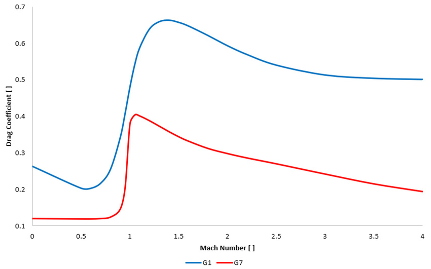
G1 was established in 1881 and models a flat-base bullet with a blunt nose. It’s still the most commonly published standard because manufacturers have used it for over a century. However, its ballistic coefficient changes significantly with velocity, making long-range predictions less reliable.

G7 was developed for modern long-range ammunition. It models a sleek, boat-tail bullet, which is what precision shooters actually use today. Because G7 coefficients stay more stable across velocities, it’s superior for anything beyond 600 yards.

If you want to dive deeper into the math, JBM Ballistics is the gold standard for free, academic-quality ballistics tools.

Eureka!

While you may think I wrote this blog to be about ballistics calculators, I also really want to share my thought process and how I figured out a way to make a meaningful performance contribution to an already solved problem. On the surface it might seem like we are limited by the speed of the processor; we have a projectile, we compute the necessary forces, then iterate the simulation to compute the projectile’s path. The key idea is that we shouldn’t be attempting to optimize our physics simulation, but rather what we want it to do.

We really only care about what the projectile is doing when it’s close to the target. Only when we approach closer and closer to the target, we start care a lot more about the accuracy of our simulation. The interesting thing is that this is exactly the same issue that graphics programmers have. When a video game uses ray marching to render objects, the color of the ray only chances when it hits a surface; everything else doesn’t matter, we only care about where and when the ray hits an object and nothing else beforehand.

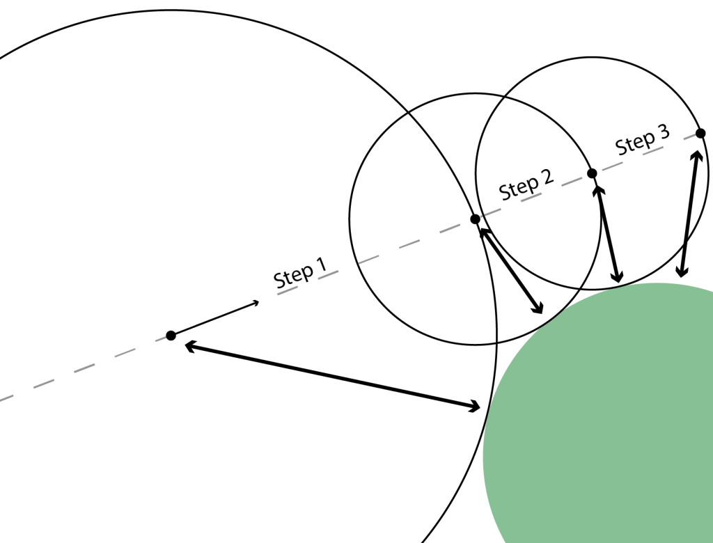
Thus, to make ray marching as efficient as possible we can take larger steps when we are away from the object, and smaller steps when we are closer, as shown in the figure above. This simple change makes the step size scale logarithmically rather than linearly to the object. The neat thing is that we can use the exact same logic to our ballistics calculator!

Making It Go Blazingly Fast

The Foundation: Rust

Before optimizing anything, we need a baseline implementation. In my case, Rust was the obvious choice for its superior combination of memory safety and performance.

Here, the ‘naive’ approach uses fixed timesteps, where the simulation is advanced by a small amount, recalculates forces, and repeats forever.

fn step(&mut self, dt: f64) {
    let drag = self.compute_drag();
    let gravity = Vec3::new(0.0, 0.0, -9.81);

    let acceleration = (drag / self.mass) + gravity;

    self.velocity += acceleration * dt;
    self.position += self.velocity * dt;
}

// Naive: fixed timestep until we reach the target
while projectile.position.x < target.x {
    projectile.step(0.0001); // ~10,000 steps per second
}

This works, but for a long trajectory you’ll need tens of thousands (if not millions) of steps for most long distance targets.

SDF-Inspired Adaptive Stepping

Here’s where the ‘ray tracing trick’ steps in. Instead of fixed timesteps, what if took longer steps when we are further from the target, and smaller ones when we are closer?

fn adaptive_step(&mut self, target: Vec3) {
    let distance = (target - self.position).magnitude();
    let speed = self.velocity.magnitude();

    // Step by half the estimated time to reach target
    let dt = 0.5 * (distance / speed);

    self.step(dt);
}

Here, we try and halve the distance to our target at every step. Even though the force calculations are almost identical, we now only compute a fraction of the trajectory.

Results

	AB Quantum	py-ballisticcalc	Ballistics-engine	libballistics	KOBE
Time	~1200ms	2320ms	63ms	26ms	0.00038ms
Drop	11.13m	17.07m	6.91m	11.14m	11.87m
Error	N/A (reference)	+53%	-38%	+0.08%	+5.4%

A 68,421x speed increase when compared to libballistics while also being the most accurate rust implementation.

The Second Side Quest: Doing more

Now that we have a performant and minimal physics simulation, we can begin making it more complicated and actually useful.

Hardware Acceleration

Because each trajectory calculation is completely independent it can be easily parallelised on a GPU.

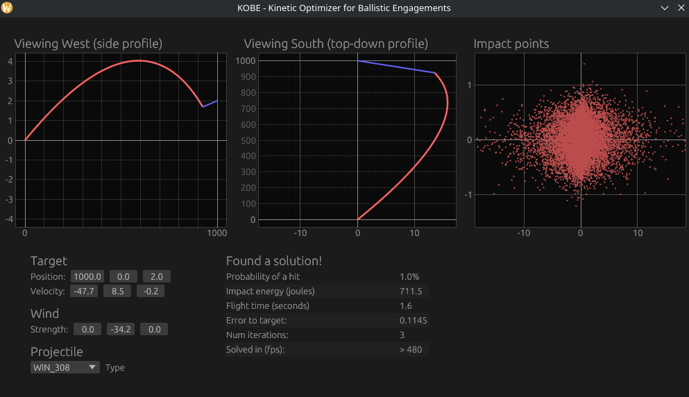
This allows us to run a far more sophisticated analysis than would ever be practical on a CPU for “free” (excluding memory overhead). This means that instead of calculating one perfect trajectory, we calculate tens of thousands with slight variations in muzzle velocity, wind estimates, and barrel condition. The result is a probability distribution of impact points rather than a single prediction, allowing us to determine the probability of hitting a given target.

Dealing with Moving Targets

Circling back to the beginning of this blog, this project was meant to simulate ballistic engagements with drones; but what if we could try and find optimal launch angles?

Unfortunately this is a bit in the technical weeds, so in brief, KOBE uses a simple ML-based technique to iteratively optimise the launch trajectory of the projectile. I found that this technique is far more efficient than something like Monte Carlo which relies on ‘spraying and praying’ that at least one simulated projectile hits the target. This also means it’s more robust at dealing with strong winds or targets that are moving extremely quickly.

Final Performance

Once we add these additional features, we can use criterion to measure final performance:

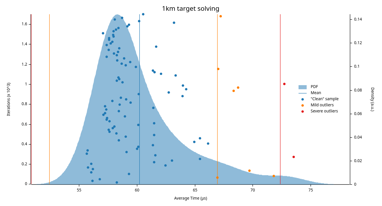
The graph above shows 100 samples of KOBE computing the ideal launch trajectory of a 7.62×51mm NATO round at a target 1km away. Despite also simulating 50,000 impacts per sample, KOBE is still 4x faster than libballistics resolving a single path.

Future work

While I believe KOBE is certainly the first of it’s kind, it still requires a target to optimise for. I’ve been playing around with zero-shot image detection but it’s still a struggle to determine distance and drone size. That being said, there might be a Part II to this blog post depending on progress 👀.

Conclusion

Ultimately this project was a massive experiment and I had a lot of fun learning about all these different technologies and how they can all satisfyingly align to solve a useful problem.

If you would like to learn more about this calculator (or even play around with it), I have a short report that might be of interest.